Quantitative Bias Analysis for Epidemiologic Data
Denis Haine
2024-03-13
Source:vignettes/episensr.Rmd
episensr.RmdQuantitative bias analysis allows to estimate nonrandom errors in epidemiologic studies, assessing the magnitude and direction of biases, and quantifying their uncertainties. Every study has some random error due to its limited sample size, and is susceptible to systematic errors as well, from selection bias to the presence of (un)known confounders or information bias (measurement error, including misclassification). Bias analysis methods were compiled by Lash et al. in their book “Applying Quantitative Bias Analysis to Epidemiologic Data”. This package implements the various bias analyses from that book, which are also available (for some) as a spreadsheet or a SAS macro, as well as some additional approaches. This vignette provides some examples on how to use the package.
Functions available in episensr are:
-
selection: Selection bias -
mbias: Selection bias caused by M bias -
confounders: Unmeasured or unknown confounders -
confounders.poly: Polytomous confounders -
confounders.emm: Unmeasured or unknown confounders in the presence of effect modification -
confounders.limit: Bounding the bias limits of unmeasured confounding -
confounders.array: Bias due to unmeasured confounders based on confounding imbalance among exposed and unexposed -
confounders.ext: Unmeasured confounders based on external measurement -
confounders.evalue: E-value due to unmeasured confounder -
misclassification: Disease or exposure misclassification -
misclassification_cov: Covariate misclassification -
bootstrap: Bootstrap resampling for selection and misclassification bias -
multidimBias: Multidimensional bias analysis -
probsens.sel: Probabilistic analysis for selection bias -
probsens.conf: Probabilistic analysis for unmeasured confounding -
probsens: Probabilistic analysis for misclassification -
probsens.irr.conf: Probabilistic analysis for unmeasured confounding of person-time data -
probsens.irr: Probabilistic analysis for exposure misclassification of person-time data -
multiple bias: Multiple bias modeling
Selection Bias
We will use a case-control study by Stang et al. on the relation between mobile phone use and uveal melanoma. The observed odds ratio for the association between regular mobile phone use vs. no mobile phone use with uveal melanoma incidence is 0.71 [95% CI 0.51-0.97]. But there was a substantial difference in participation rates between cases and controls (94% vs 55%, respectively) and so selection bias could have an impact on the association estimate. The 2X2 table for this study is the following:
| Regular use | No use | |
|---|---|---|
| Cases | 136 | 107 |
| Controls | 297 | 165 |
We use the function selection as shown below.
## Loading required package: ggplot2## Thank you for using episensr!## This is version 1.3.0 of episensr## Type 'citation("episensr")' for citing this R package in publications.
stang <- selection(matrix(c(136, 107, 297, 165),
                          dimnames = list(c("UM+", "UM-"), c("Mobile+", "Mobile-")),
                          nrow = 2, byrow = TRUE),
                   bias_parms = c(.94, .85, .64, .25))
stang
## --Observed data--
## Outcome: UM+
## Comparing: Mobile+ vs. Mobile-
##
## Mobile+ Mobile-
## UM+ 136 107
## UM- 297 165
##
## 2.5% 97.5%
## Observed Relative Risk: 0.7984287 0.6518303 0.9779975
## Observed Odds Ratio: 0.7061267 0.5143958 0.9693215
## ---
##
## Selection Bias Corrected Relative Risk: 1.483780
## Selection Bias Corrected Odds Ratio: 1.634608The various episensr functions return an object which is
a list containing the input and output variables. You can check it out
with str().
The 2X2 table is provided as a matrix and selection probabilities
given with the argument bias_parms, a vector with the 4
probabilities (guided by the participation rates in cases and controls)
in the following order: among cases exposed, among cases unexposed,
among noncases exposed, and among noncases unexposed. The output shows
the observed 2X2 table and the observed odds ratio (and relative risk),
followed by the corrected ones.
Misclassification Bias
Misclassification bias can be assessed with the function
misclassification. Confidence intervals for corrected
association due to exposure misclassification are also directly
available, or the estimates can also be bootstrapped (see below). The
confidence intervals from the variance of the corrected odds ratio
estimator in the misclassification function are computed as
in Greenland et al.
and Chu et
al., when adjusting for exposure misclassification using sensitivity
and specificity. Using the example in Chu et al. of a case-control study
of cigarette smoking and invasive pneumococcal disease, the unadjusted
odds ratio is 4.32, with a 95% confidence interval of 2.96 to 6.31.
Let’s say the sensitivity of self-reported smoking is 94% and
specificity is 97%, for both the case and control groups:
misclassification(matrix(c(126, 92, 71, 224),
                         dimnames = list(c("Case", "Control"),
                                         c("Smoking +", "Smoking - ")),
                         nrow = 2, byrow = TRUE),
                  type = "exposure",
                  bias_parms = c(0.94, 0.94, 0.97, 0.97))
## --Observed data--
## Outcome: Case
## Comparing: Smoking + vs. Smoking -
##
## Smoking + Smoking -
## Case 126 92
## Control 71 224
##
## 2.5% 97.5%
## Observed Relative Risk: 2.196866 1.796016 2.687181
## Observed Odds Ratio: 4.320882 2.958402 6.310846
## ---
## 2.5% 97.5%
## Misclassification Bias Corrected Relative Risk: 2.377254
## Misclassification Bias Corrected Odds Ratio: 5.024508 3.282534 7.690912The corrected odds ratio is now 5.02, with a widened 95% confidence interval (3.28 to 7.69). Note the bias despite the large sensitivity and specificity.
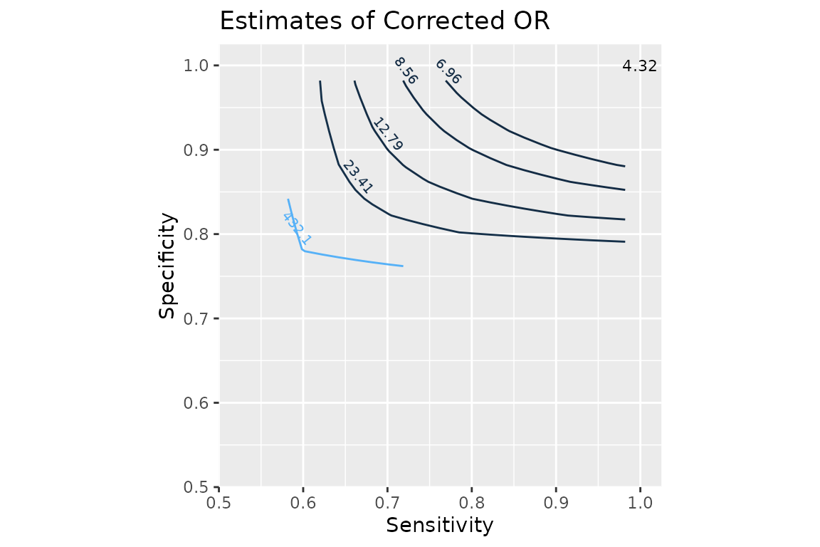
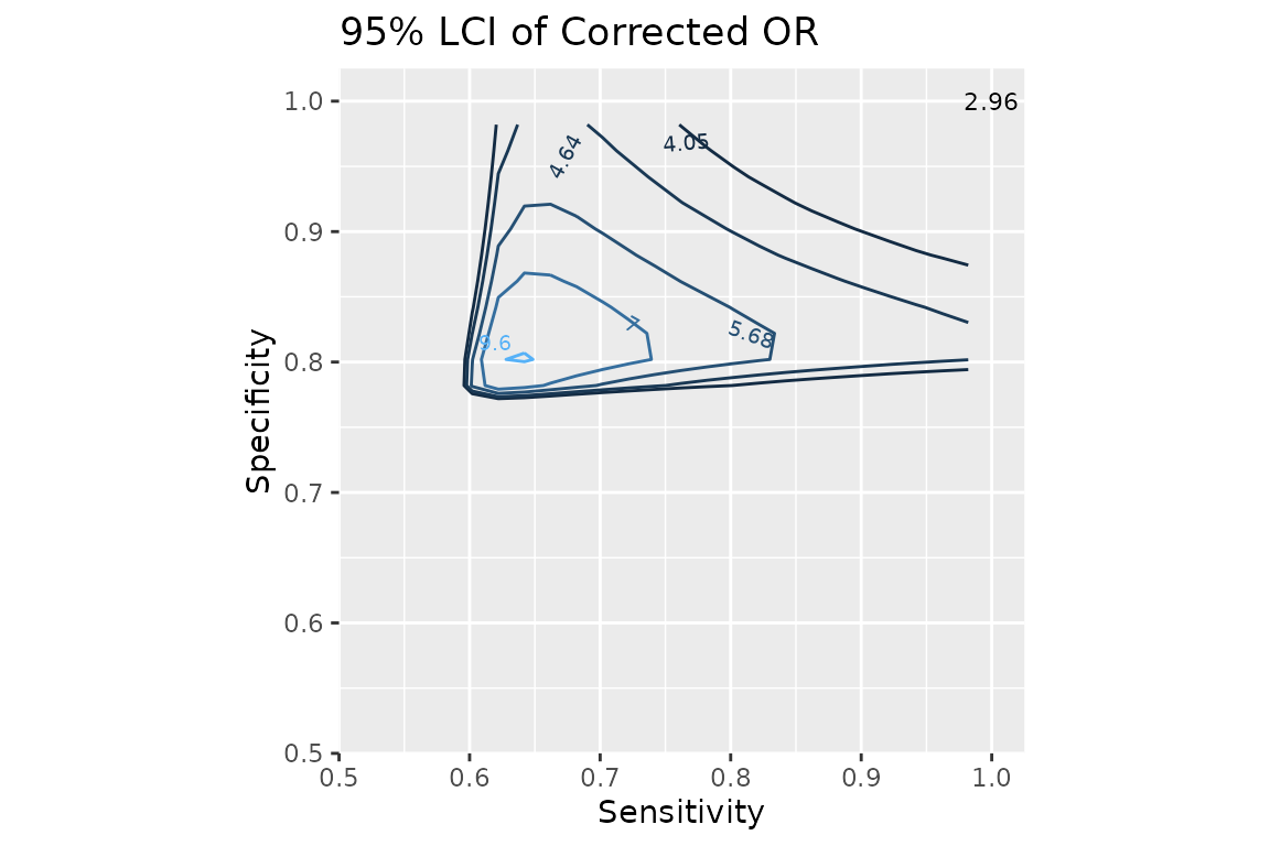
You can even reproduce the contour plots in Chu et al. paper!
dat <- expand.grid(Se = seq(0.582, 1, 0.02),
                   Sp = seq(0.762, 1, 0.02))

dat$OR_c <- apply(dat, 1,
                  function(x) misclassification(matrix(c(126, 92, 71, 224),
                                                       nrow = 2, byrow = TRUE),
                                                type = "exposure",
                                                bias_parms = c(x[1], x[1], x[2], x[2]))$adj.measures[2, 1])
dat$OR_c <- round(dat$OR_c, 2)

library(ggplot2)
library(directlabels)
p1 <- ggplot(dat, aes(x = Se, y = Sp, z = OR_c)) +
    geom_contour(aes(colour = ..level..), breaks = c(4.32, 6.96, 8.56, 12.79, 23.41, 432.1)) +
    annotate("text", x = 1, y = 1, label = "4.32", size = 3) +
    scale_fill_gradient(limits = range(dat$OR_c), high = 'red', low = 'green') +
    scale_x_continuous(breaks = seq(0.5, 1, .1), expand = c(0,0)) +
    scale_y_continuous(breaks = seq(0.5, 1, .1), expand = c(0,0)) +
    coord_fixed(ylim = c(0.5, 1.025), xlim = c(0.5, 1.025)) +
    scale_colour_gradient(guide = 'none') +
    xlab("Sensitivity") +
    ylab("Specificity") +
    ggtitle("Estimates of Corrected OR")
direct.label(p1, list("far.from.others.borders", "calc.boxes", "enlarge.box",
                      hjust = 1, vjust = -.5, box.color = NA, cex = .6,
                      fill = "transparent", "draw.rects"))
Contour plot of point estimates of corrected odds ratio (OR)
dat$ORc_lci <- apply(dat, 1,
                     function(x) misclassification(matrix(c(126, 92, 71, 224),
                                                          nrow = 2, byrow = TRUE),
                                                   type = "exposure",
                                                   bias_parms = c(x[1], x[1], x[2], x[2]))$adj.measures[2, 2])
dat$ORc_lci <- round(dat$ORc_lci, 2)

p3 <- ggplot(dat, aes(x = Se, y = Sp, z = ORc_lci)) +
    geom_contour(aes(colour = ..level..),
                 breaks = c(4.05, 4.64, 5.68, 7.00, 9.60)) +
    annotate("text", x = 1, y = 1, label = "2.96", size = 3) +
    scale_fill_gradient(limits = range(dat$ORc_lci), high = 'red', low = 'green') +
    scale_x_continuous(breaks = seq(0.5, 1, .1), expand = c(0,0)) +
    scale_y_continuous(breaks = seq(0.5, 1, .1), expand = c(0,0)) +
    coord_fixed(ylim = c(0.5, 1.025), xlim = c(0.5, 1.025)) +
    scale_colour_gradient(guide = 'none') +
    xlab("Sensitivity") +
    ylab("Specificity") +
    ggtitle("95% LCI of Corrected OR")
direct.label(p3, list("far.from.others.borders", "calc.boxes", "enlarge.box",
                           hjust = 1, vjust = -.5, box.color = NA, cex = .6,
                           fill = "transparent", "draw.rects"))
Contour plot of 95% lower confidence limit of corrected OR
The bias analysis for exposure misclassification can also use positive and negative predictive values. Bodnar et al. evaluated the accuracy of maternal prepregnancy BMI and gestational weight gain (GWG) data derived from the Pennsylvania state birth certificates against information collected from the medical record. To estimate positive and negative predictive values, a validation study was conducted by randomly sampling women conditional on their reported BMI category and term/preterm status. BMI was obtained from medical records for these sampled women and used as a gold standard for BMI category, allowing to determine positive and negative predictive values: PPVD1 = 65%, PPVD0 = 74%, NPVD1 = 100%, NPVD0 = 98%. The analysis is the following.
misclassification(matrix(c(599, 4978, 31175, 391851),
                         dimnames = list(c("Preterm", "Term"), c("Underweight", "Normal weight")),
                         nrow = 2, byrow = TRUE),
                  type = "exposure_pv",
                  bias_parms = c(0.65, 0.74, 1, 0.98))
## --Observed data--
## Outcome: Preterm
## Comparing: Underweight vs. Normal weight
##
## Underweight Normal weight
## Preterm 599 4978
## Term 31175 391851
##
## 2.5% 97.5%
## Observed Relative Risk: 1.502808 1.381743 1.634480
## Observed Odds Ratio: 1.512469 1.388465 1.647547
## ---
## 2.5% 97.5%
## Misclassification Bias Corrected Relative Risk: 0.9528156
## Misclassification Bias Corrected Odds Ratio: 0.9522211Note that using predictive values relates to the prevalence of the true exposure status, which might not be the same in every populations.
Covariate misclassification is available via the function
misclassification.cov. For example, the paper by Berry et al. looked
if misclassification of the confounding variable in vitro
fertilization (IVF), a confounder, resulted wrongly on an
association between increase folic acid and having twins. IVF increases
the risk of twins, and women undergoing IVF might be more likely to take
folic acid supplements, i.e. IVF would be a confounder between vitamins
and twins. Data on IVF were not available and a proxy for it was used,
period of involuntary childlessness. However, it was a poor
proxy for IVF, with a sensitivity of 60% and a specificity of 95%. These
bias parameters were assumed to be nondifferential. Here’s the code with
episensr:
misclassification.cov(array(c(1319, 38054, 5641, 405546, 565, 3583,
                              781, 21958, 754, 34471, 4860, 383588),
                            dimnames = list(c("Twins+", "Twins-"),
                                            c("Folic acid+", "Folic acid-"),
                                            c("Total", "IVF+", "IVF-")),
                            dim = c(2, 2, 3)),
                      bias_parms = c(.6, .6, .95, .95))
## --Observed data--
## Outcome: Twins+
## Comparing: Folic acid+ vs. Folic acid-
##
## , , Total
##
## Folic acid+ Folic acid-
## Twins+ 1319 5641
## Twins- 38054 405546
##
## , , IVF+
##
## Folic acid+ Folic acid-
## Twins+ 565 781
## Twins- 3583 21958
##
## , , IVF-
##
## Folic acid+ Folic acid-
## Twins+ 754 4860
## Twins- 34471 383588
##
##
## 2.5% 97.5%
## Observed Relative Risk: 2.441910 2.301898 2.590437
## Observed Odds Ratio: 2.491888 2.344757 2.648251
## ---
## Observed Corrected
## SMR RR adjusted for confounder: 2.261738 1.000235
## RR due to confounding by misclassified confounder: 1.079661 2.441337
## Mantel-Haenszel RR adjusted for confounder: 2.228816 1.000187
## MH RR due to confounding by misclassified confounder: 1.095608 2.441452
## SMR OR adjusted for confounder: 2.337898 1.000304
## OR due to confounding by misclassified confounder: 1.065867 2.491131
## Mantel-Haenszel OR adjusted for confounder: 2.290469 1.000215
## MH OR due to confounding by misclassified confounder: 1.087938 2.491351While the non-adjusted analysis showed that women taking folic acid were 2.44 times more likely to have twins, after correcting for the misclassification of IVF, risk ratio is now null (= 1.0).
Uncontrolled Confounders
We will use data from a cross-sectional study by Tyndall et al. on the association between male circumcision and the risk of acquiring HIV, which might be confounded by religion. The code to account for unmeasured or unknown confounders is the following, where the 2X2 table is given as a matrix. We choose a risk ratio implementation, provide a vector defining the risk ratio associating the confounder with the disease, and the prevalence of the confounder, religion, among the exposed and the unexposed.
tyndall <- confounders(matrix(c(105, 85, 527, 93),
                              dimnames = list(c("HIV+", "HIV-"), c("Circ+", "Circ-")),
                              nrow = 2, byrow = TRUE),
                       type = "RR",
                       bias_parms = c(.63, .8, .05))
tyndall
## --Observed data--
## Outcome: HIV+
## Comparing: Circ+ vs. Circ-
##
## Circ+ Circ-
## HIV+ 105 85
## HIV- 527 93
##
## 2.5% 97.5%
## Crude Relative Risk: 0.3479151 0.2757026 0.4390417
## Relative Risk, Confounder +: 0.4850550
## Relative Risk, Confounder -: 0.4850550
## ---
## RR_conf
## Standardized Morbidity Ratio: 0.4850550 0.7172695
## Mantel-Haenszel: 0.4850550 0.7172695The output gives the crude 2X2 table, the crude relative risk and confounder specific measures of association between exposure and outcome, and the relationship adjusted for the unknown confounder, using a standardized morbidity ratio (SMR) or a Mantel-Haenszel (MH) estimate of the risk ratio.
Additional information are also available, like the 2X2 tables by levels of the confounder.
## Confounder +
tyndall$cfder.data
## Circ+ Circ-
## HIV+ 75.17045 2.727967
## HIV- 430.42955 6.172033
## Confounder -
tyndall$nocfder.data
## Circ+ Circ-
## HIV+ 29.82955 82.27203
## HIV- 96.57045 86.82797As described in this function’s help file, the bias correction used is the “relative risk due to confounding” as proposed by Miettinen (Components of the crude risk ratio, Am J Epidemiol 1972, 96(2):168-172). The two examples shown in that paper are the following.
The first one is about drug surveillance data analyzed as a cohort study, with the frequency of drug-attributed rash in relation to allopurinol exposure among recipients of ampicillin, with sex treated as a potential confounding factor.
rash <- matrix(c(15, 94, 52, 1163),
               dimnames = list(c("Rash +", "Rash -"),
                               c("Allopurinol +", "Allopurinol -")),
nrow = 2, byrow = TRUE)| Allopurinol + | Allopurinol - | |
|---|---|---|
| Rash + | 15 | 94 |
| Rash - | 52 | 1163 |
We can decompose these numbers by confounders:
## Outcome by confounders
rash_conf <- matrix(c(36, 58, 645, 518),
                    dimnames = list(c("Rash +", "Rash -"),
                                    c("Males", "Females")),
                    nrow = 2, byrow = TRUE)
## By confounders: among males
rash_males <- matrix(c(5, 36, 33, 645),
                     dimnames = list(c("Rash +", "Rash -"),
                                     c("Allopurinol +", "Allopurinol -")),
                     nrow = 2, byrow = TRUE)
## By confounders: among females
rash_females <- matrix(c(10, 58, 19, 518),
                       dimnames = list(c("Rash +", "Rash -"),
                                       c("Allopurinol +", "Allopurinol -")),
nrow = 2, byrow = TRUE)| Males | Females | |
|---|---|---|
| Rash + | 36 | 58 |
| Rash - | 645 | 518 |
| Allopurinol + | Allopurinol - | |
|---|---|---|
| Rash + | 5 | 36 |
| Rash - | 33 | 645 |
| Allopurinol + | Allopurinol - | |
|---|---|---|
| Rash + | 10 | 58 |
| Rash - | 19 | 518 |
And then get the bias parameters:
(RR_no <- (36/(36+645))/(58/(58+518))) # RR between confounder and outcome among non-exposed## [1] 0.5249886
(p1 <- (5+33)/(15+52)) # prevalence of confounder among exposed## [1] 0.5671642
(p2 <- (36+645)/(94+1163)) # prevalence of confounder among unexposed## [1] 0.5417661With the following results:
rash %>% confounders(., type = "RR", bias_parms = c(RR_no, p1, p2))## --Observed data--
## Outcome: Rash +
## Comparing: Allopurinol + vs. Allopurinol -
##
## Allopurinol + Allopurinol -
## Rash + 15 94
## Rash - 52 1163
##
## 2.5% 97.5%
## Crude Relative Risk: 2.993808 1.840724 4.869218
## Relative Risk, Confounder +: 3.043245
## Relative Risk, Confounder -: 3.043245
## ---
## RR_conf
## Standardized Morbidity Ratio: 3.0432448 0.9837551
## Mantel-Haenszel: 3.0432448 0.9837551For the second example, data are from a case-control study of the relationship of oral contraceptive use to venous thrombosis with age as a confounding factor.
thromb <- matrix(c(12, 30, 53, 347),
                 dimnames = list(c("Thrombosis +", "Thrombosis -"),
                                 c("OC +", "OC -")),
nrow = 2, byrow = TRUE)| OC + | OC - | |
|---|---|---|
| Thrombosis + | 12 | 30 |
| Thrombosis - | 53 | 347 |
## Outcome by confounders
thromb_conf <- matrix(c(18, 12, 158, 189),
                      dimnames = list(c("Thrombosis +", "Thrombosis -"),
                                      c("20-29 years old", "30-39 years old")),
                      nrow = 2, byrow = TRUE)
## By confounders: among 20-29 years old
thromb_younger <- matrix(c(10, 18, 39, 158),
                       dimnames = list(c("Thrombosis +", "Thrombosis -"),
                                       c("OC +", "OC -")),
                       nrow = 2, byrow = TRUE)
## By confounders: among 30-39 years old
thromb_older <- matrix(c(2, 12, 14, 189),
                     dimnames = list(c("Thrombosis +", "Thrombosis -"),
                                     c("OC +", "OC -")),
nrow = 2, byrow = TRUE)| 20-29 years old | 30-39 years old | |
|---|---|---|
| Thrombosis + | 18 | 12 |
| Thrombosis - | 158 | 189 |
| OC + | OC - | |
|---|---|---|
| Thrombosis + | 10 | 18 |
| Thrombosis - | 39 | 158 |
| OC + | OC - | |
|---|---|---|
| Thrombosis + | 2 | 12 |
| Thrombosis - | 14 | 189 |
And then the bias parameters:
(OR_no <- (18/12)/(158/189)) # OR between confounder and outcome among non-exposed## [1] 1.794304
(p1 <- (10+39)/(12+53)) # prevalence of confounder among exposed## [1] 0.7538462
(p2 <- (18+158)/(30+347)) # prevalence of confounder among unexposed## [1] 0.4668435With the following results:
thromb %>% confounders(., type = "OR", bias_parms = c(OR_no, p1, p2))## --Observed data--
## Outcome: Thrombosis +
## Comparing: OC + vs. OC -
##
## OC + OC -
## Thrombosis + 12 30
## Thrombosis - 53 347
##
## 2.5% 97.5%
## Crude Odds Ratio: 2.618868 1.263076 5.429973
## Odds Ratio, Confounder +: 2.245449
## Odds Ratio, Confounder -: 2.245449
## ---
## OR_conf
## Standardized Morbidity Ratio: 2.245449 1.166300
## Mantel-Haenszel: 2.245449 1.166300Bootstrapping
Selection and misclassification bias models can be bootstrapped in order to get confidence interval on the adjusted association parameter. We can use the ICU dataset from Hosmer and Lemeshow Applied Logistic Regression textbook as an example. The replicates that give negative cells in the adjusted 2X2 table are silently ignored and the number of effective bootstrap replicates is provided in the output. Ten thousands bootstrap samples are a good number for testing everything runs smoothly. But again, don’t be afraid of running more, like 100,000 bootstrap samples.
library(aplore3)  # to get ICU data
data(icu)

## First run the model
misclass_eval <- misclassification(icu$sta, icu$inf,
                                   type = "exposure",
                                   bias_parms = c(.75, .85, .9, .95))
misclass_eval
## --Observed data--
## Outcome: Died
## Comparing: Yes vs. No
##
## exposed
## case Yes No
## Died 24 16
## Lived 60 100
##
## 2.5% 97.5%
## Observed Relative Risk: 2.071429 1.175157 3.651272
## Observed Odds Ratio: 2.500000 1.230418 5.079573
## ---
## 2.5% 97.5%
## Misclassification Bias Corrected Relative Risk: 3.627845
## Misclassification Bias Corrected Odds Ratio: 4.871795 1.235506 19.210258
## Then bootstrap it
set.seed(123)
misclass_boot <- boot.bias(misclass_eval, R = 10000)
misclass_boot
## 95 % confidence interval of the bias adjusted measures:
## RR: 0.9595117 11.96789
## OR: 1.075386 19.44271
## ---
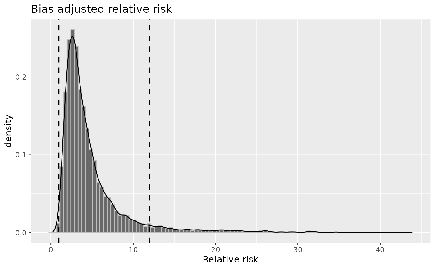
## Based on 9562 bootstrap replicatesBootstrap replicates can also be plotted, with the confidence interval shown as dotted lines.
plot(misclass_boot, "rr")
Bootstrap replicates and confidence interval.