Probabilistic Sensitivity Analysis
Denis Haine
2024-03-13
Source:vignettes/b_probabilistic.Rmd
b_probabilistic.RmdBias parameters are not always known. A probabilistic sensitivity
analysis allows to specify a probability distribution for the bias
parameters and then, through Monte Carlo sampling, to generate a
frequency distribution of the corrected estimates of effect.
episensr has a set of probsens functions for
this:
-
probsens.sel: Probabilistic analysis for selection bias -
probsens.conf: Probabilistic analysis for unmeasured confounding -
probsens: Probabilistic analysis for misclassification -
probsens.irr.conf: Probabilistic analysis for unmeasured confounding of person-time data -
probsens.irr: Probabilistic analysis for exposure misclassification of person-time data
The available distributions for the various bias parameters throughout these functions are:
- Constant,
- Uniform,
- Triangular,
- Trapezoidal,
- Logit-logistic,
- Logit-normal, and
- Beta.
Probabilistic Sensitivity Analysis for Exposure Misclassification
We use a study on the effect of smoking during pregnancy on breast
cancer risk by Fink
& Lash, where we assume nondifferential misclassification of the
exposure, smoking, with probability density functions for sensitivities
(Se) and specificities (Sp) among cases and noncases equal to uniform
distributions with a minimum of 0.7 and a maximum of 0.95 for
sensitivities (0.9 and 0.99 respectively for specificities). We choose
to correct for exposure misclassification with the argument
type = exposure. We ask for 50000 replications (default is
1000). Don’t be shy with the number of iterations, episensr is fast.
The Se and Sp for cases (seca, spca) are
given as a list with its first element referring to the type of
distribution (choice between constant, uniform, triangular, trapezoidal,
logit-logistic, and logit-normal) and the second element giving the
distribution parameters (min and max for uniform distribution). By
avoiding to provide information on the noncases (seexp,
spexp), we are referring to a nondifferential
misclassification.
## Loading required package: ggplot2## Thank you for using episensr!## This is version 1.3.0 of episensr## Type 'citation("episensr")' for citing this R package in publications.
set.seed(123)
smoke.nd <- probsens(matrix(c(215, 1449, 668, 4296),
                            dimnames = list(c("BC+", "BC-"), c("Smoke+", "Smoke-")),
                            nrow = 2, byrow = TRUE),
                     type = "exposure",
                     reps = 50000,
                     seca.parms = list("uniform", c(.7, .95)),
                     spca.parms = list("uniform", c(.9, .99)))
smoke.nd
## --Observed data--
## Outcome: BC+
## Comparing: Smoke+ vs. Smoke-
##
## Smoke+ Smoke-
## BC+ 215 1449
## BC- 668 4296
##
## 2.5% 97.5%
## Observed Relative Risk: 0.9653825 0.8523766 1.0933704
## Observed Odds Ratio: 0.9542406 0.8092461 1.1252141
## ---
## Median 2.5th percentile
## Relative Risk -- systematic error: 0.9431650 0.8817325
## Odds Ratio -- systematic error: 0.9253996 0.8478414
## Relative Risk -- systematic and random error: 0.9359816 0.8175818
## Odds Ratio -- systematic and random error: 0.9162763 0.7664183
## 97.5th percentile
## Relative Risk -- systematic error: 0.9612154
## Odds Ratio -- systematic error: 0.9487841
## Relative Risk -- systematic and random error: 1.0690389
## Odds Ratio -- systematic and random error: 1.0923026The output gives the 2X2 table, the observed measures of association, and the corrected measures of association.
We saved the probsens analysis in a new object
smoke.nd. We can see its elements with the function
str():
str(smoke.nd)## List of 8
## $ obs.data : num [1:2, 1:2] 215 668 1449 4296
## ..- attr(*, "dimnames")=List of 2
## .. ..$ : chr [1:2] "BC+" "BC-"
## .. ..$ : chr [1:2] "Smoke+" "Smoke-"
## $ obs.measures: num [1:2, 1:3] 0.965 0.954 0.852 0.809 1.093 ...
## ..- attr(*, "dimnames")=List of 2
## .. ..$ : chr [1:2] " Observed Relative Risk:" " Observed Odds Ratio:"
## .. ..$ : chr [1:3] " " "2.5%" "97.5%"
## $ adj.measures: num [1:4, 1:3] 0.943 0.925 0.936 0.916 0.882 ...
## ..- attr(*, "dimnames")=List of 2
## .. ..$ : chr [1:4] " Relative Risk -- systematic error:" " Odds Ratio -- systematic error:" "Relative Risk -- systematic and random error:" " Odds Ratio -- systematic and random error:"
## .. ..$ : chr [1:3] "Median" "2.5th percentile" "97.5th percentile"
## $ sim.df :'data.frame': 50000 obs. of 12 variables:
## ..$ seca : num [1:50000] 0.772 0.897 0.802 0.921 0.935 ...
## ..$ seexp : num [1:50000] 0.772 0.897 0.802 0.921 0.935 ...
## ..$ spca : num [1:50000] 0.919 0.94 0.912 0.943 0.965 ...
## ..$ spexp : num [1:50000] 0.919 0.94 0.912 0.943 0.965 ...
## ..$ A1 : num [1:50000] 117 137 95 139 174 ...
## ..$ B1 : num [1:50000] 1547 1527 1569 1525 1490 ...
## ..$ C1 : num [1:50000] 386 442 321 446 548 ...
## ..$ D1 : num [1:50000] 4578 4522 4643 4518 4416 ...
## ..$ corr.RR: num [1:50000] 0.918 0.94 0.905 0.943 0.954 ...
## ..$ corr.OR: num [1:50000] 0.893 0.922 0.877 0.925 0.94 ...
## ..$ tot.RR : num [1:50000] 0.903 1.067 0.854 1.056 0.999 ...
## ..$ tot.OR : num [1:50000] 0.873 1.09 0.812 1.075 0.999 ...
## $ reps : num 50000
## $ fun : chr "probsens"
## $ warnings : NULL
## $ message : NULL
## - attr(*, "class")= chr [1:3] "episensr" "episensr.probsens" "list"smoke.nd is a list of 8 elements where different
information on the analysis done are saved. We have
smoke.nd$obs.data where we have the observed 2X2 table,
smoke.nd$obs.measures (the observed measures of
association), smoke.nd$adj.measures (the adjusted measures
of association), and smoke.nd$sim.df, a data frame with the
simulated variables from each replication, like the Se and Sp, the 4
cells of the adjusted 2X2 table, and the adjusted measures.
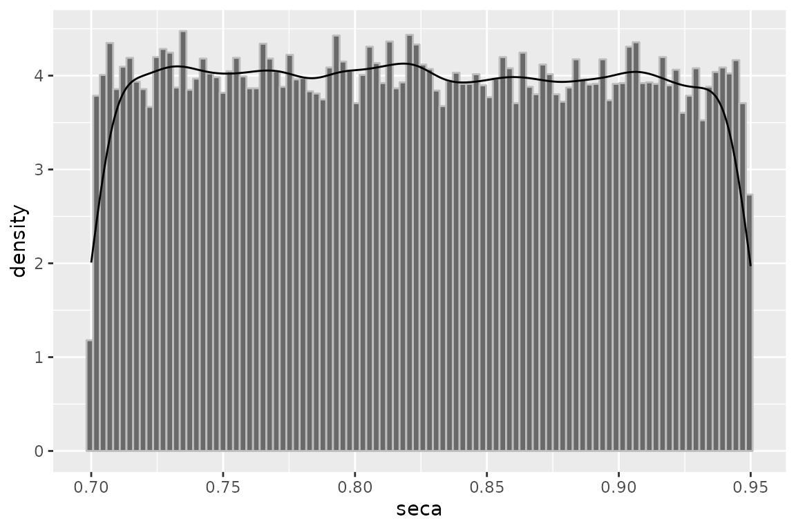
episensr offers some plot functions to allow plotting
directly these saved information, for example the Se prior
distribution:
plot(smoke.nd, "seca")
Sensibility prior distribution.
There are combinations of Se, Sp, and disease (or exposure) prevalence that can produce negative cells in the corrected 2-by-2 table. For outcome misclassification, this happen when the frequency of observed exposed cases is less than the total number of diseased individuals multiplied by the false-positive proportion. Negative cell counts occur when the false-positive proportion is greater than the proportion of cases that are exposed. When providing values for Se and Sp that are more or less like random classification (i.e. Se ~50% and Sp ~50%), you can obtain negative cell values.
Note that a message is provided if the chosen distribution(s) lead to
negative cell values, with the number of iterations affected. By
default, these iterations are deleted from the simulation. However, user
can keep these iterations which will be set to zero by setting
discard to FALSE. It is recommended to shift
distributions upwards if more than 10% of the iterations are deleted (Fox et al., 2005).
Probabilistic Sensitivity Analysis for Uncontrolled Confounding
Let’s illustrate this function with this example where the association between occupational resins exposure and lung cancer mortality is studied, together with the presence of an unmeasured potential confounder, smoking (Greenland et al., 1994).
| Resins exposed | Resins unexposed | |
|---|---|---|
| Cases | 45 | 94 |
| Controls | 257 | 945 |
After adjustment for age and year at death, Greenland et al. found an OR of 1.77 (95% CI from 1.18 to 2.64). Is smoking, for which they had no data about, had an effect on this association? How large the association between resins and smoking had to be to remove the association between resins and lung cancer association after adjustment for smoking? For this, you have to know 3 bias parameters: the association between smoking and lung cancer, the prevalence of smoking among those unexposed to resins, and the prevalence of smoking in those exposed to resins.
Prior probability distributions are given to each bias parameters. Prevalences of smoking in those exposed to resins, and of smoking in those unexposed to resins receive prior distributions that are uniform between 0.40 and 0.70. Prior distribution for the odds ratio associating smoking with lung cancer mortality is log-normal with 95% limits of 5 and 15. The mean of this distribution is [ln(15) + ln(5)] / 2 = 2.159, and its standard deviation is [ln(15) - ln(5)] / 3.92 = 0.28. It looks like this:
##      2.5%     97.5%
##  4.979672 14.959055
Log-normal distribution with meanlog = 2.159 and sdlog = 0.28.
Now, let’s run probsens.conf with 50,000 iterations:
set.seed(123)
greenland <- probsens.conf(matrix(c(45, 94, 257, 945),
                                  dimnames = list(c("Cases+", "Cases-"), c("Res+", "Res-")),
                                  nrow = 2, byrow = TRUE),
                           reps = 50000,
                           prev.exp = list("uniform", c(.4, .7)),
                           prev.nexp = list("uniform", c(.4, .7)),
                           risk = list("log-normal", c(2.159, .28)))
greenland
## --Observed data--
## Outcome: Cases+
## Comparing: Res+ vs. Res-
##
## Res+ Res-
## Cases+ 45 94
## Cases- 257 945
##
## 2.5% 97.5%
## Observed Relative Risk: 1.646999 1.182429 2.294094
## Observed Odds Ratio: 1.760286 1.202457 2.576898
## ---
## Median 2.5th percentile
## RR (SMR) -- systematic error: 1.648388 1.166250
## RR (SMR) -- systematic and random error: 1.645768 1.018201
## OR (SMR) -- systematic error: 1.841387 1.209338
## OR (SMR) -- systematic and random error: 1.841158 1.041488
## 97.5th percentile
## RR (SMR) -- systematic error: 2.325654
## RR (SMR) -- systematic and random error: 2.670214
## OR (SMR) -- systematic error: 2.822182
## OR (SMR) -- systematic and random error: 3.278307The median adjusted OR is 1.84 [1.21,2.82]. The ratio of the two 95% CI bounds is 2.82/1.21 = 2.33. The ratio from the conventional 95% confidence limits was 2.57/1.20 = 2.14. These 2 ratios are pretty close, and therefore our uncertainty about confounding is similar to our uncertainty about random error.
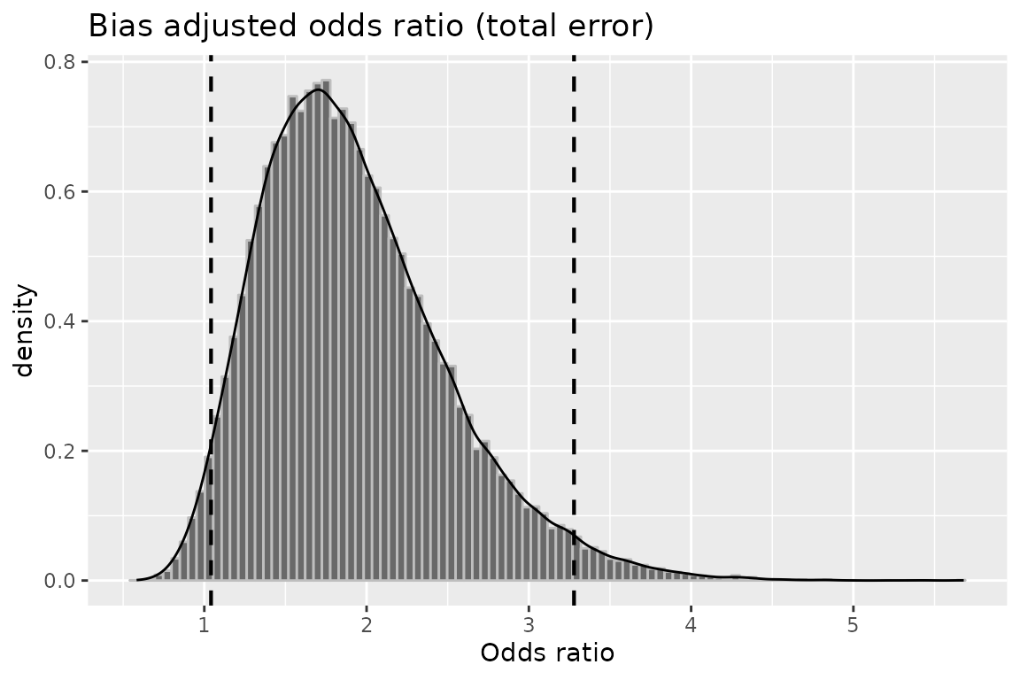
You can plot the bias-adjusted OR including both systematic and random error:
plot(greenland, "or_tot")
Distribution of the 50,000 confounder-adjusted odds ratios.