Learning the apply family of functions

One of the greatest joys of vectorized operations is being able to use the entire family of apply functions that are available in base R.

These include:

apply
by
lapply
tapply
sapply

apply

apply applies a function to each row or column of a matrix. It's a convenient way to get marginal values. It follows this syntax: apply(object, dimension, function).

m <- matrix(c(1:10, 11:20), nrow = 10, ncol = 2)
m

      [,1] [,2]
 [1,]    1   11
 [2,]    2   12
 [3,]    3   13
 [4,]    4   14
 [5,]    5   15
 [6,]    6   16
 [7,]    7   17
 [8,]    8   18
 [9,]    9   19
[10,]   10   20

# 1 is the row index
# 2 is the column index
apply(m, 1, sum)  # row totals

 [1] 12 14 16 18 20 22 24 26 28 30

apply(m, 2, sum)  # column totals

[1]  55 155

apply(m, 1, mean)

 [1]  6  7  8  9 10 11 12 13 14 15

apply(m, 2, mean)

[1]  5.5 15.5

There are convenience functions based on apply: rowSums(x), colSums(x), rowMeans(x), colMeans(x), addmargins.

by

by applies a function to subsets of a data frame.

by(prod.long$milk, prod.long[, "test"], summary)

prod.long[, "test"]: 1
   Min. 1st Qu.  Median    Mean 3rd Qu.    Max.    NA's 
  10.40   26.00   33.00   33.41   40.90   59.20     135 
-------------------------------------------------------- 
prod.long[, "test"]: 10
   Min. 1st Qu.  Median    Mean 3rd Qu.    Max.    NA's 
   5.20   16.50   21.60   21.78   25.90   45.30     332 
-------------------------------------------------------- 
prod.long[, "test"]: 2
   Min. 1st Qu.  Median    Mean 3rd Qu.    Max.    NA's 
   9.40   27.70   34.40   35.05   41.90   60.30     141 
-------------------------------------------------------- 
prod.long[, "test"]: 3
   Min. 1st Qu.  Median    Mean 3rd Qu.    Max.    NA's 
   3.80   25.20   32.00   32.86   39.00   64.50     158 
-------------------------------------------------------- 
prod.long[, "test"]: 4
   Min. 1st Qu.  Median    Mean 3rd Qu.    Max.    NA's 
  10.00   24.00   30.50   31.29   38.58   57.60     174 
-------------------------------------------------------- 
prod.long[, "test"]: 5
   Min. 1st Qu.  Median    Mean 3rd Qu.    Max.    NA's 
  10.10   22.10   29.80   29.74   36.10   54.20     199 
-------------------------------------------------------- 
prod.long[, "test"]: 6
   Min. 1st Qu.  Median    Mean 3rd Qu.    Max.    NA's 
  10.00   22.30   28.40   28.43   34.60   54.80     219 
-------------------------------------------------------- 
prod.long[, "test"]: 7
   Min. 1st Qu.  Median    Mean 3rd Qu.    Max.    NA's 
   9.70   20.22   26.55   26.71   32.70   52.50     234 
-------------------------------------------------------- 
prod.long[, "test"]: 8
   Min. 1st Qu.  Median    Mean 3rd Qu.    Max.    NA's 
   4.20   19.08   25.20   24.95   30.13   46.90     252 
-------------------------------------------------------- 
prod.long[, "test"]: 9
   Min. 1st Qu.  Median    Mean 3rd Qu.    Max.    NA's 
   5.00   18.20   23.00   23.10   27.05   45.50     285

Exercise 1

Using by, what is the mean milk production for each monthly test? (use the prod.long dataset)

Solution

by(prod.long$milk, prod.long[, "test"], function(x) mean(x, na.rm = TRUE))

tapply

tapply applies a function to subsets of a vector.

tapply(health.wide$age, health.wide$lactation, mean)

        1         2         3         4         5         6         7 
 2.234899  3.372519  4.447423  5.574000  6.663043  7.457143  8.685714 
        8         9 
 9.825000 10.100000

tapply() returns an array; by()returns a list.

lapply (and llply)

What it does: Returns a list of same length as the input. Each element of the output is a result of applying a function to the corresponding element.

my_list <- list(a = 1:10, b = 2:20)
my_list

$a
 [1]  1  2  3  4  5  6  7  8  9 10

$b
 [1]  2  3  4  5  6  7  8  9 10 11 12 13 14 15 16 17 18 19 20

lapply(my_list, mean)

$a
[1] 5.5

$b
[1] 11

sapply

sapply is a more user friendly version of lapply and will return a list of matrix where appropriate.

Let's work with the same list we just created.

my_list

$a
 [1]  1  2  3  4  5  6  7  8  9 10

$b
 [1]  2  3  4  5  6  7  8  9 10 11 12 13 14 15 16 17 18 19 20

x <- sapply(my_list, mean)
x

   a    b 
 5.5 11.0

class(x)

[1] "numeric"

replicate

An extremely useful function to generate datasets for simulation purposes.

replicate(10, rnorm(10))

             [,1]        [,2]         [,3]        [,4]        [,5]
 [1,] -0.18296801 -0.07941687  0.556866478  0.32202953  0.49421349
 [2,]  1.02546237  0.23094961 -0.027725896 -1.33510987 -0.36789050
 [3,]  0.61763429  0.27703658 -0.633289121  0.97164947 -1.24375323
 [4,] -0.78905915  0.32296508  0.590272159  1.31506326  1.41135827
 [5,] -0.51034496  0.63508227  2.055402761 -0.89659294 -0.28714015
 [6,] -0.37624329  0.78419520 -1.205187780 -0.29507644  1.32026833
 [7,]  0.08537509  1.86086714 -0.970240977  0.07661003 -2.25080168
 [8,] -0.14789145  1.57162130 -0.007669854 -0.05094117 -0.02900168
 [9,] -0.26309675  0.86304561 -0.733189759 -0.03084748 -1.61350051
[10,] -0.05618467  0.89226587 -1.266500283 -0.59140376  1.02791954
            [,6]        [,7]        [,8]        [,9]      [,10]
 [1,]  0.4426889  0.03526615 -0.90270328 -0.26814034  0.5401839
 [2,]  1.0911277 -0.08477494  0.39941108  0.82335054  0.2204077
 [3,]  0.5253514  0.19089756  0.97723529 -1.72851775  0.1809154
 [4,] -0.9069135 -0.79663168 -0.69463126  0.05781333  0.6269190
 [5,]  1.0669793 -3.08790009  0.69193494 -0.67787888 -1.0643246
 [6,] -1.3896023 -0.30786629 -0.82441093 -1.09917333  0.6365318
 [7,]  1.1329454 -1.44655598  0.35700710  0.58868047 -1.1802607
 [8,] -1.1190632 -0.90202972  0.59884816 -0.57900125  0.4512936
 [9,]  1.1162238  1.03717790  0.41516267 -0.14242241  0.1062566
[10,]  1.9634481 -1.18035318 -0.02035708 -0.81575567 -0.5582405

replicate(10, rnorm(10), simplify = TRUE)

             [,1]        [,2]       [,3]        [,4]       [,5]
 [1,] -0.54746727  0.71188242 -0.7692378  0.20776940 -1.1911955
 [2,]  0.17129389  1.17065806  0.7341176 -0.19784111  1.4999466
 [3,]  1.09769758 -0.04547800  0.5835762 -1.98329516 -0.5509973
 [4,]  0.49039424 -1.58614965  1.7075941 -0.48315885  0.7405964
 [5,]  0.33509901  0.38512102 -0.7831752  0.28508535  0.2430618
 [6,]  0.92131753 -0.15772011 -0.4985644  0.00217137  0.5447922
 [7,] -0.01576046  0.11304573 -0.6274871 -0.25288329 -0.2649672
 [8,]  1.73799532  0.02527156  0.3225937 -1.67327665 -1.0400179
 [9,] -0.97862588  0.62199262  1.0316596 -0.62823981  0.3306254
[10,] -0.66175684 -0.53292217 -1.0175170 -1.70367106  0.8996907
             [,6]        [,7]       [,8]         [,9]        [,10]
 [1,]  0.20172680  0.39767985 -1.4565158  0.343714295  0.608689123
 [2,] -0.09933205 -0.82269883  0.2607614 -0.913100277 -0.731100767
 [3,] -1.64026535 -1.34769622  0.1357663 -1.348551922 -1.287339421
 [4,]  0.46878069 -1.44551108  1.8891981 -0.456134156  0.001269542
 [5,] -0.13024399  0.79899685 -1.0435204 -0.413426122 -1.458832823
 [6,] -1.02578585  0.01650778  0.3144996 -1.103240123 -0.650437291
 [7,] -0.98625566 -1.01259025  2.4682385 -0.585127293 -1.051062421
 [8,] -0.22434056  0.31500438 -0.1349445 -0.082358386  1.120358846
 [9,]  1.60622386 -1.34955072 -0.1424986 -0.454433715 -1.773935613
[10,]  0.44464687 -0.38118115  1.0751461 -0.009772592  1.328939639

The final arguments turns the result into a vector or matrix if possible.

mapply

Its more or less a multivariate version of sapply. It applies a function to all corresponding elements of each argument.

example:

list_1 <- list(a = c(1:10), b = c(11:20))
list_1

$a
 [1]  1  2  3  4  5  6  7  8  9 10

$b
 [1] 11 12 13 14 15 16 17 18 19 20

list_2 <- list(c = c(21:30), d = c(31:40))
list_2

$c
 [1] 21 22 23 24 25 26 27 28 29 30

$d
 [1] 31 32 33 34 35 36 37 38 39 40

mapply(sum, list_1$a, list_1$b, list_2$c, list_2$d)

 [1]  64  68  72  76  80  84  88  92  96 100

apply functions are more computationally efficient than loops
you could also use reshape2 and plyr/dplyr packages

aggregate

aggregate(age ~ lactation + da, data = health.wide, FUN = mean)

   lactation  da       age
1          1  No  2.235862
2          2  No  3.366667
3          3  No  4.417582
4          4  No  5.572917
5          5  No  6.668889
6          6  No  7.457143
7          7  No  8.816667
8          8  No  9.825000
9          9  No 10.100000
10         1 Yes  2.200000
11         2 Yes  3.750000
12         3 Yes  4.900000
13         4 Yes  5.600000
14         5 Yes  6.400000
15         7 Yes  7.900000

table

t1 <- table(health.wide$parity)
t1


  1  2+ 
149 351

t2 <- table(health.wide$parity, health.wide$da)
t2

prop.table(t1)


    1    2+ 
0.298 0.702

prop.table(t2)

    
        No   Yes
  1  0.290 0.008
  2+ 0.678 0.024

prop.table(t2, margin = 2)

    
            No       Yes
  1  0.2995868 0.2500000
  2+ 0.7004132 0.7500000

See also xtabs(), ftable() or CrossTable() (in library gmodels).

Exercise 2

From the lesson on R objects, you created a matrix based on the following: Three hundred and thirty-three cows are milked by a milker wearing gloves and 280 by a milker not wearing gloves. Two hundred cows in each group developed a mastitis. Using the apply family of functions, find out the risk ratio and odds ratio for mastitis according to wearing gloves.

	Mastitis	No mastitis
Gloves	: 200 :	: 133 :
No gloves	: 200 :	: 80 :

Solution

tab <- rbind(c(200, 133), c(200, 80))
rownames(tab) <- c("Gloves", "No gloves")
colnames(tab) <- c("Mastitis", "No mastitis")

row.tot <- apply(tab, 1, sum)
risk <- tab[, "Mastitis"] / row.tot
risk.ratio <- risk / risk[2]
odds <- risk / (1 - risk)
odds.ratio <- odds / odds[2]
rbind(risk, risk.ratio, odds, odds.ratio)

              Gloves No gloves
risk       0.6006006 0.7142857
risk.ratio 0.8408408 1.0000000
odds       1.5037594 2.5000000
odds.ratio 0.6015038 1.0000000

Split-Apply-Combine in Action

The following figure can give you a sense of what is split-apply-combine.

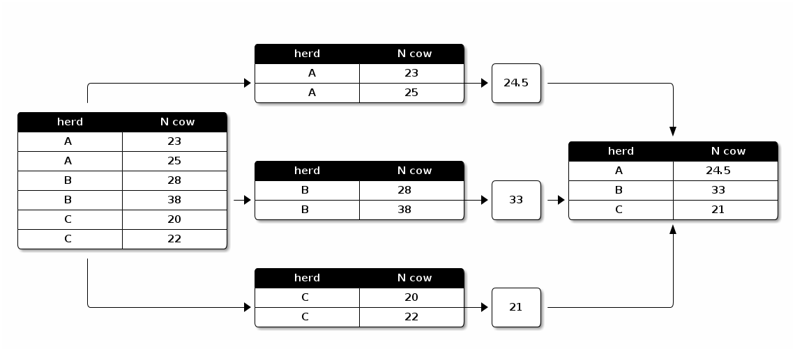
plyr package can be used to apply the split-apply-combine strategy. You need to provide the following information:

The data structure of the input
The dataset being worked on
The variable to split the dataset on.
The function to apply to each split piece.
The data structure of the output to combine pieces.

In short, plyr synthetizes the entire *apply family. For example, the mean age by herd and parity could be computed and saved into a data frame:

lact <- ddply(health.wide,
              .(herd, parity),
              summarize,
              mean.age = mean(age)
              )

Two other packages can also be helpful in applying this strategyL dplyr and data.table.