R Objects / Data Structure
-
To make the best of the R language, you'll need a strong understanding of the basic data types and data structures and how to operate on those.
-
Very Important to understand because these are the objects you will manipulate on a day-to-day basis in R. Dealing with object conversions is one of the most common sources of frustration for beginners.
-
Everything in
Ris an object.
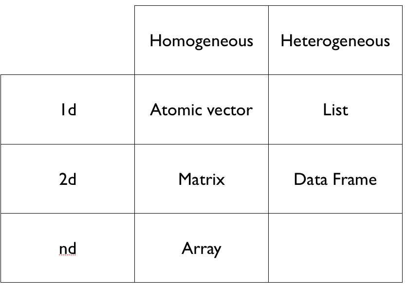
R has many different structures for storing the data you want to analyze. The most commonly used are
- vectors
- lists
- matrices
- arrays
- data frames
It can be determined with the function class().
The type or mode of an object defines how it is stored. It could be
- a character,
- a numeric value,
- an integer,
- a complex number, or
- a logical value (Boolean value: TRUE/FALSE).
It can be determined with the function typeof(). length() informs you about
its size and attributes() if the object has any metadata associated to it.
| Example | Type |
|---|---|
| "a", "swc" | character |
| 2, 15.5 | numeric |
2 (Must add a L at end to denote integer) |
integer |
TRUE, FALSE |
logical |
| 1+4i | complex |
x <- "dataset"
typeof(x)
[1] "character"
attributes(x)NULL
y <- 1:10
typeof(y)
[1] "integer"
length(y)[1] 10
z <- c(1L, 2L, 3L)
typeof(z)
[1] "integer"
Below is a short definition and quick example of each of these data structures which you can use to decide which is the best for representing your data in R.
Vector
It is the most basic data type. Vectors only have one dimension and
all their elements must be the same mode. There are various ways to
create vectors. The simplest one is with the c function.
x <- c(1, 2, 5)
x
[1] 1 2 5
length(x)[1] 3
x is a numeric vector. These are the most common kind. They are numeric
objects and are treated as double precision real numbers. To explicitly create
integers, add an L at the end.
x1 <- c(1L, 2L, 5L)You can also have logical vectors.
y <- c(TRUE, TRUE, FALSE, FALSE)Finally you can have character vectors:
z <- c("Holstein", "Brown Swiss", "Jersey")The c function allows to combine its arguments. If the arguments
are of various modes, they will be reduced to their lowest common
type:
x2 <- c(1, 3, "a")
x2
[1] "1" "3" "a"
typeof(x2)[1] "character"
This is called implicit coercion. Objects can be explicitly coerced with the
as.<class_name> function.
as.character(x1)[1] "1" "2" "5"
You can also use the : operator or the seq function:
1:10 [1] 1 2 3 4 5 6 7 8 9 10
seq(from = 5, to = 25, by = 5)[1] 5 10 15 20 25
Other objects
Inf is infinity. You can have either positive or negative infinity.
1/0[1] Inf
1/Inf[1] 0
NaN means Not a number. It's an undefined value.
0/0[1] NaN
Each object can have attributes. Attributes can be part of an object of R. These include:
- names
- dimnames
- dim
- class
- attributes (contain metadata)
Matrix
A matrix is a rectangular array of numbers. Technically, it is a
vector with two additional attributes: number of rows and number of
columns. This is what you would use to analyze a spreadsheet full of
only numbers, or only words. You can create a matrix with the matrix
function:
m <- rbind(c(1, 4), c(2, 2))
m
[,1] [,2]
[1,] 1 4
[2,] 2 2
m <- cbind(c(1, 4), c(2, 2))
m
[,1] [,2]
[1,] 1 2
[2,] 4 2
dim(m)[1] 2 2
m <- matrix(data = 1:12, nrow = 4, ncol = 3,
            dimnames = list(c("cow1", "cow2", "cow3", "cow4"),
                c("milk", "fat", "prot")))
m
milk fat prot
cow1 1 5 9
cow2 2 6 10
cow3 3 7 11
cow4 4 8 12
Matrices are filled column-wise but you can also use the byrow argument to
specify how the matrix is filled.
m <- matrix(1:12, nrow = 4, ncol = 3, byrow = TRUE,
            dimnames = list(c("cow1", "cow2", "cow3", "cow4"),
                c("milk", "fat", "prot")))
m
milk fat prot
cow1 1 2 3
cow2 4 5 6
cow3 7 8 9
cow4 10 11 12
List
A list is an ordered collection of objects where the objects can be of different modes.
l <- list("a", "b", "c", TRUE, 4)Each element of a list can be given a name and referred to by that name. Elements of a list can be accessed by their number or their name.
cow <- list(breed = "Holstein", age = 3, last.prod = c(25, 35, 32))
cow$breed
[1] "Holstein"
cow[[1]][1] "Holstein"
Lists can be used to hold together multiple values returned from a function. For example the elements used to create an histogram can be saved and returned:
h <- hist(islands)
str(h)List of 6
$ breaks : num [1:10] 0 2000 4000 6000 8000 10000 12000 14000 16000 18000
$ counts : int [1:9] 41 2 1 1 1 1 0 0 1
$ density : num [1:9] 4.27e-04 2.08e-05 1.04e-05 1.04e-05 1.04e-05 ...
$ mids : num [1:9] 1000 3000 5000 7000 9000 11000 13000 15000 17000
$ xname : chr "islands"
$ equidist: logi TRUE
- attr(*, "class")= chr "histogram"
The function str() is used here. It stands for structure and shows
the internal structure of an R object.
Factor
Factor is a special type of vector to store categorical values. They can be
ordered or unordered and are important for modelling functions such as
lm() and glm(), and also in plot methods.
Factors can only contain pre-defined values.
Factors are pretty much integers that have labels on them. While factors look (and often behave) like character vectors, they are actually integers under the hood, and you need to be careful when treating them like strings. Some string methods will coerce factors to strings, while others will throw an error.
Sometimes factors can be left unordered. Example: male, female.
Other times you might want factors to be ordered (or ranked). Example: low,
medium, high.
Underlying it is represented by numbers 1, 2, 3.
They are better than using simple integer labels because factors are what are
called self describing. male and female is more descriptive than 1s and
2s. Helpful when there is no additional metadata.
Which is male? 1 or 2? You wouldn't be able to tell with just integer
data. Factors have this information built in.
Factors can be created with factor(). Input is generally a character vector.
breed <- factor(c("Holstein", "Holstein", "Brown Swiss", "Holstein",
                  "Ayrshire", "Canadian", "Canadian", "Brown Swiss",
                  "Holstein", "Brown Swiss", "Holstein"))
breed
[1] Holstein Holstein Brown Swiss Holstein Ayrshire
[6] Canadian Canadian Brown Swiss Holstein Brown Swiss
[11] Holstein
Levels: Ayrshire Brown Swiss Canadian Holstein
It stores values as a set of labelled integers. Some functions treat factors differently from numeric vectors.
table(breed)breed
Ayrshire Brown Swiss Canadian Holstein
1 3 2 5
If you need to convert a factor to a character vector, simply use
as.character(breed) [1] "Holstein" "Holstein" "Brown Swiss" "Holstein" "Ayrshire"
[6] "Canadian" "Canadian" "Brown Swiss" "Holstein" "Brown Swiss"
[11] "Holstein"
In modelling functions, it is important to know what the baseline level is.
This is the first factor but by default the ordering is determined by
alphabetical order of words entered. You can change this by specifying the
levels (another option is to use the function relevel()).
x <- factor(c("yes", "no", "yes"), levels = c("yes", "no"))
x
[1] yes no yes
Levels: yes no
Array
If a matrix is a two-dimensional data structure, we can add layers
to the data and have further dimensions in addition to rows and
columns. These datasets would be arrays. It can be
created with the array function:
a <- array(data = 1:24, dim = c(3, 4, 2))Data frame
Data frames are used to store tabular data: multiple rows, columns and format.
Data frames can have additional attributes such as rownames(), which can be
useful for annotating data, like subject_id or sample_id. But most of the time
they are not used.
Some additional information on data frames:
-
Usually created by
read.csv()andread.table(). -
Can convert to
matrixwithdata.matrix() -
Coercion will be forced and not always what you expect.
-
Can also create with
data.frame()function. -
Find the number of rows and columns with
nrow(df)andncol(df), respectively. -
Rownames are usually 1..n.
df <- data.frame(cow = c("Moo-Moo", "Daisy", "Elsie"),
                 prod = c(35, 40, 28),
                 pregnant = c(TRUE, FALSE, TRUE))
Combining data frames
cbind(df, data.frame(z = 4)) cow prod pregnant z
1 Moo-Moo 35 TRUE 4
2 Daisy 40 FALSE 4
3 Elsie 28 TRUE 4
When you combine column wise, only row numbers need to match. If you are adding a vector, it will get repeated.
Useful functions
head()- see first 6 rowstail()- see last 6 rowsdim()- see dimensionsnrow()- number of rowsncol()- number of columnsstr()- structure of each columnnames()- will list thenamesattribute for a data frame (or any object really), which gives the column names.
A data frame is a special type of list where every element of the list has same length.
See that it is actually a special list:
is.list(df)[1] TRUE
class(df)[1] "data.frame"
Missing values
Denoted by NA and/or NaN for undefined mathematical operations.
is.na()
is.nan()
Check for both.
NA values have a class. So you can have both an integer NA (NA_integer_) and a
character NA (NA_character_).
NaN is also NA. But not the other way around.
x <- c(1, 2, NA, 4, 5)
x
[1] 1 2 NA 4 5
is.na(x) # returns logical[1] FALSE FALSE TRUE FALSE FALSE
# shows third
is.nan(x)
[1] FALSE FALSE FALSE FALSE FALSE
# none are NaNx <- c(1, 2, NA, NaN, 4, 5)
is.na(x)[1] FALSE FALSE TRUE TRUE FALSE FALSE
# shows 2 TRUE
is.nan(x)
[1] FALSE FALSE FALSE TRUE FALSE FALSE
# shows 1 TRUEExercise 1
Import the health dataset. This dataset presents the lactations of
500 cows from various herds, providing age, lactation number, presence of milk
fever (mf) and/or displaced abomasum (da) coded as 0/1. Have a look at the
different variables. What type are they? Would you like to convert any of them
to a factor variable? How would you do it? How would you create a variable parity
categorizing lactation into the categories 1, 2+ (hint: see ?cut)? check
that it creates factors.
Solution
health <- read.csv(
    file = "health.csv",
    header = TRUE,
    stringsAsFactors = FALSE)

str(health)
'data.frame': 1000 obs. of 5 variables:
$ unique : chr "K100-P284" "K100-P284" "K100-P295" "K100-P295" ...
$ age : num 6.7 6.7 6.9 6.9 5.9 5.9 6.6 6.6 5.4 5.4 ...
$ lactation: int 6 6 6 6 4 4 5 5 4 4 ...
$ disease : chr "mf" "da" "mf" "da" ...
$ presence : int 0 0 0 0 0 0 0 0 0 0 ...
health$presence <- factor(health$presence, labels = c("No", "Yes"))
health$parity <- cut(health$lactation,
                     breaks = c(0, 1, max(health$lactation)),
                     labels = c("1", "2+"))
Exercise 2
Three hundred and thirty-three cows are milked by a milker wearing gloves and
280 by a milker not wearing gloves. Two hundred cows in each group developed a
mastitis. Create the following table and perform a chi-squared test (hint:
chisq.test).
| Mastitis | No mastitis | |
|---|---|---|
| Gloves | : 200 : | : 133 : |
| No gloves | : 200 : | : 80 : |
Solution
tab <- rbind(c(200, 133), c(200, 80))
rownames(tab) <- c("Gloves", "No gloves")
colnames(tab) <- c("Mastitis", "No mastitis")
tab
Mastitis No mastitis
Gloves 200 133
No gloves 200 80
chisq.test(tab)
	Pearson's Chi-squared test with Yates' continuity correction

data:  tab
X-squared = 8.1761, df = 1, p-value = 0.004245
Review of R data types